Understanding Matrix Operations from a Geometric Perspective

Unlike functions, matrices provide another way of organizing and operating on numbers or symbols. This raises several questions:

• If we already have functions, why do we need matrices?
• How are matrices and functions different, and how are they related (as two of the most fundamental mathematical tools)?
• What do abstract matrix operations actually mean, either physically or in the real world?

At present, I still cannot fully answer these questions, especially this one: functions and matrices are two fundamental “data structures” for describing relationships between quantities and how those relationships change, but what is the essential connection—and distinction—between them?

Symmetry Between Matrix Rows and Columns?

The rows and columns of a matrix are symmetric in many respects. For example, determinants satisfy $|A|=|A^T|$, and row rank equals column rank. At the same time, rows and columns are asymmetric in many other respects. For example, matrix multiplication generally satisfies $AB\ne BA$, and when solving systems of equations, we can only use row operations.

Why? Each individual question appears to have its own answer. But why? These should not be several unrelated, isolated facts; there ought to be a more general reason behind them.

Sometimes this reminds me of our left and right hands. Are they symmetric? They are symmetric in one sense, but asymmetric in another: no translation or rotation can make one hand coincide with the other. A similar phenomenon appears in the molecular structures studied in chemistry. Although the rows and columns of a matrix possess a natural symmetry, our definition of matrix multiplication introduces an asymmetry (otherwise, $AB$ would be commutative).

This leads to another question: Why do different multiplication orders have different definitions? What real-world meaning lies behind this? Does it imply that matrix rows and columns are inherently asymmetric?

My current answer is that we must distinguish left from right. The same is true for the rows and columns of a matrix: we need to define operations on row vectors differently from operations on column vectors. That convention is matrix multiplication, and the distinction between left and right multiplication—together with the question of which object the matrix acts on—captures the difference between row and column operations. For example, $AB$ can be viewed either as $A$ multiplying $B$ from the left or as $B$ multiplying $A$ from the right, while in a system of equations it can only be interpreted in one of these ways.

Because of the definition of matrix multiplication, consider right multiplication as an example of a column transformation:

1. Write the matrix on the left in terms of its column vectors:

$$[\boldsymbol{\alpha}_1,\boldsymbol{\alpha}_2,\ldots,\boldsymbol{\alpha}_n]K = [\boldsymbol{\beta}_1,\boldsymbol{\beta}_2,\ldots,\boldsymbol{\beta}_m].$$

Then

$$\boldsymbol{\beta}_j=\sum_{i=1}^{n}k_{ij}\boldsymbol{\alpha}_i.$$

Here, the entries $k_{ij}$ of $K=(k_{ij})$ are scalars, while all the other quantities are vectors.

We can see that right-multiplying a collection of column vectors by a matrix produces another collection of column vectors, and each $\boldsymbol{\beta}$ is a linear combination of the original $\boldsymbol{\alpha}$ vectors.

2. Now write the matrix on the left in terms of its row vectors:

$$\begin{bmatrix} \boldsymbol{\alpha}_1\\ \boldsymbol{\alpha}_2\\ \vdots\\ \boldsymbol{\alpha}_n \end{bmatrix}K = \begin{bmatrix} \boldsymbol{\beta}_1\\ \boldsymbol{\beta}_2\\ \vdots\\ \boldsymbol{\beta}_n \end{bmatrix}, \qquad (\boldsymbol{\beta}_i)_j =\boldsymbol{\alpha}_i\cdot \begin{bmatrix}k_{1j}\\k_{2j}\\\vdots\\k_{nj}\end{bmatrix}.$$

A problem now becomes apparent: the $\boldsymbol{\beta}$ vectors cannot be written as linear combinations of the $\boldsymbol{\alpha}$ vectors, and their relationship becomes more complicated.

Comparing the two representations above, it is not difficult to see that the difference comes precisely from the rule that the upper-left entry of a product is obtained by taking the inner product of the first row of the matrix on the left with the first column of the matrix on the right. This naturally creates an asymmetry between left and right, making the distinction between left and right multiplication easier to understand.

P.S. Suppose we changed the rule for matrix multiplication. For example, in $AB=C$, imagine defining the upper-left entry of $C$ as the inner product of the first column of $A$ with the first row of $B$, with all other entries defined correspondingly. The result would then be reversed.

P.P.S. The discussion above only uses “right multiplication produces a column transformation” as an example. The statement that left multiplication produces a row transformation follows by analyzing the matrix on the right; readers may verify this themselves.

Why Does the “Acting Matrix” Sometimes Appear on the Left and Sometimes on the Right of a Set of Column Vectors?

1. When expressing or transforming a set of vectors, the column vectors appear on the left, while the acting matrix $C$ appears on the right:

If $\boldsymbol{\eta}_1,\boldsymbol{\eta}_2,\ldots,\boldsymbol{\eta}_n$ and $\boldsymbol{\xi}_1,\boldsymbol{\xi}_2,\ldots,\boldsymbol{\xi}_n$ are two bases of $\mathbb{R}^n$, then there exists a transition matrix $C=(c_{ij})_{n\times n}$ such that

$$[\boldsymbol{\eta}_1,\boldsymbol{\eta}_2,\ldots,\boldsymbol{\eta}_n] = [\boldsymbol{\xi}_1,\boldsymbol{\xi}_2,\ldots,\boldsymbol{\xi}_n]C.$$

2. In an eigenvalue problem, the eigenvectors form a collection of column vectors, while the acting matrix $A$ appears on the left:

$$A[\boldsymbol{\xi}_1,\boldsymbol{\xi}_2,\ldots,\boldsymbol{\xi}_n] = [\boldsymbol{\xi}_1,\boldsymbol{\xi}_2,\ldots,\boldsymbol{\xi}_n] \operatorname{diag}(\lambda_1,\lambda_2,\ldots,\lambda_n).$$

Different Ways of Viewing Matrix Operations

In the previous section, I discussed matrix multiplication from the perspective of representing a set of vectors and explained the idea of “left for rows, right for columns.” But the issue is not that simple. What is a transformation? In the equation above, each $\vec{\xi_i}$ is transformed by $A$ into $\lambda_i\vec{\xi_i}$. Is that not also a transformation?

There are therefore two ways to transform a set of vectors:

1. Treat the set of vectors as a whole. Each transformed vector can be expressed linearly in terms of the original collection of vectors, and all the coefficients together form the transformation matrix $C$.
2. Treat the set of vectors merely as a “collection” whose members are independent of one another. Each transformed vector is obtained by applying $A$ to the corresponding original vector.

In the first equation, $C$ is the coefficient matrix used in the first kind of transformation. In the second equation, $A$ is the matrix used to find the eigenvectors and acts as the transformation in the second sense.

---

But this is not the end of the story: from another perspective, $C$ is $A$!

---

Consider the following example. $\alpha$ is a vector—that is, a collection of coordinates. In three-dimensional space, for example,

$$\vec{\alpha}=\begin{bmatrix}1\\1\\1\end{bmatrix}.$$

Suppose I have a “transformation matrix” $C$ that rotates the $y$-axis of the original coordinate system by $180^\circ$:

$$C=\begin{bmatrix}1&0&0\\0&-1&0\\0&0&1\end{bmatrix}.$$

As for why $C$ takes this form, readers can verify it and review elementary transformation matrices. What, then, is $\alpha'$ in the new coordinate system? Clearly, the $y$-coordinate becomes negative:

$$\vec{\alpha'} =\begin{bmatrix}1\\-1\\1\end{bmatrix} =C\vec{\alpha} =\begin{bmatrix}1&0&0\\0&-1&0\\0&0&1\end{bmatrix} \begin{bmatrix}1\\1\\1\end{bmatrix}.$$

Here, $\alpha$ corresponds to the $\vec{\xi_i}$ in the equation above. In the change-of-basis equation, however, the same $C$ becomes the transformation-coefficient matrix and moves to the right of the column-vector set. The difference is that the column-vector set is now treated as a whole—a basis. In the following equation, $x$ gives the coordinates of $\alpha$ in one basis, while $y$ gives its coordinates in another:

$$\boldsymbol{\alpha} =[\boldsymbol{\xi}_1,\boldsymbol{\xi}_2,\ldots,\boldsymbol{\xi}_n]\boldsymbol{x} =[\boldsymbol{\eta}_1,\boldsymbol{\eta}_2,\ldots,\boldsymbol{\eta}_n]\boldsymbol{y}.$$

If the transition matrix from the basis $\boldsymbol{\xi}_1,\ldots,\boldsymbol{\xi}_n$ to the basis $\boldsymbol{\eta}_1,\ldots,\boldsymbol{\eta}_n$ is $C$, then

$$[\boldsymbol{\eta}_1,\ldots,\boldsymbol{\eta}_n] =[\boldsymbol{\xi}_1,\ldots,\boldsymbol{\xi}_n]C, \qquad \boldsymbol{x}=C\boldsymbol{y}, \qquad \boldsymbol{y}=C^{-1}\boldsymbol{x}.$$

A change of basis is also easy to understand. In the example above, the three basis vectors $\vec{i}$, $\vec{j}$, and $\vec{k}$ of the original coordinate system are

$$\vec{i}=\begin{bmatrix}1\\0\\0\end{bmatrix}, \quad \vec{j}=\begin{bmatrix}0\\1\\0\end{bmatrix}, \quad \vec{k}=\begin{bmatrix}0\\0\\1\end{bmatrix}, \quad \vec{\alpha}=1\vec{i}+1\vec{j}+1\vec{k} =\begin{bmatrix}1\\1\\1\end{bmatrix}.$$

The transformation by $C$ is

$$[\vec{i'},\vec{j'},\vec{k'}] =[\vec{i},\vec{j},\vec{k}]C, \quad\text{that is,}\quad \begin{bmatrix}1&0&0\\0&-1&0\\0&0&1\end{bmatrix} = \begin{bmatrix}1&0&0\\0&1&0\\0&0&1\end{bmatrix} \begin{bmatrix}1&0&0\\0&-1&0\\0&0&1\end{bmatrix}.$$

This simple example should make the apparently abstract process of changing bases and coordinates easier to understand.

Summary

So is it really “left for rows, right for columns”? Why does it sometimes seem otherwise? From the perspective of vector spaces, we can see the complete picture very clearly: it—the transformation matrix—is still the same thing; only our perspective has changed.

The transformation matrix used for a basis transformation and the transformation matrix used for a coordinate transformation are “the same.” But when it transforms a “basis” as a set and when it transforms a set of “coordinates,” we understand it from different perspectives, so naturally it sometimes appears on the left and sometimes on the right. More details about transformation matrices will be discussed in the next section.

Viewing Matrices Through Coordinate-System Transformations

In a fixed coordinate system, $A_{n\times n}\alpha=\beta$ first means that the matrix $A$ applies a linear transformation to the vector $\alpha$, producing the vector $\beta$. When $A$ is invertible, it maps one basis of the original space to another basis. We can therefore also understand $A$ as applying an invertible transformation to the entire $n$-dimensional space. If we regard the transformed basis as a new basis, then $A$ also determines the relationship between the old and new coordinate systems. Note that $A\alpha=\beta$ describes an active transformation of a vector, whereas converting the coordinates of the same vector between the old and new coordinate systems usually involves $A^{-1}$. This extends the discussion of vector-space transformations in the previous section, “Different Ways of Viewing Matrix Operations.”

Invertible and Non-Invertible Transformations

An invertible matrix performs an invertible transformation of an $n$-dimensional coordinate system without losing information, whereas a transformation by a non-invertible matrix cannot be undone:

Suppose an unknown vector $\alpha$ is transformed into $\beta$ through $A\alpha=\beta$, and both the invertible matrix $A$ and the vector $\beta$ are known. Then the original $\alpha$ can always be recovered. If $A$ is not invertible, however, $\alpha$ cannot be recovered.

In other words, after an invertible transformation $A$, any two distinct vectors remain distinct; after a non-invertible transformation $B$, there must be two distinct vectors that are transformed into the same vector.

Projection

A projection is a special kind of non-invertible coordinate transformation. For example, projecting the three-dimensional vector $\alpha=(x,y,z)$ onto the $x$-axis can be written as $A\alpha=\beta$, where

$$\begin{bmatrix}1&0&0\\0&0&0\\0&0&0\end{bmatrix} \begin{bmatrix}x\\y\\z\end{bmatrix} = \begin{bmatrix}x\\0\\0\end{bmatrix}.$$

Flipping / Reflection

As in the example in the previous section, reflecting the coordinate space across the $xOz$ plane reverses the $y$-axis:

$$\begin{bmatrix}1&0&0\\0&-1&0\\0&0&1\end{bmatrix} \begin{bmatrix}x\\y\\z\end{bmatrix} = \begin{bmatrix}x\\-y\\z\end{bmatrix}.$$

Scaling

Scaling is somewhat similar to reflection: it stretches or compresses the basis vector corresponding to a particular direction in an orthogonal basis. For example, suppose we compress the sphere $x^2+y^2+z^2=1$ along the $z$-axis to form an ellipsoid. Then

$$\begin{bmatrix}1&0&0\\0&1&0\\0&0&\frac{1}{2}\end{bmatrix} \begin{bmatrix}x\\y\\z\end{bmatrix} = \begin{bmatrix}x\\y\\\frac{z}{2}\end{bmatrix}.$$

Rotation

This is where the famously “terrifying” orthogonal matrix comes from. Suppose we preserve the scale of the original space and only rotate it. What properties must the transformation matrix have?

$$\begin{bmatrix}a_{11}&a_{12}&a_{13}\\a_{21}&a_{22}&a_{23}\\a_{31}&a_{32}&a_{33}\end{bmatrix} \begin{bmatrix}x\\y\\z\end{bmatrix} = \begin{bmatrix}x'\\y'\\z'\end{bmatrix}.$$

• The lengths of the vectors (coordinates) before and after the transformation must remain unchanged.

The Connection Between Coordinate Transformations and Calculus

A “complex” surface is often transformed from a simple one, such as a sphere. This reveals that a transformation is essentially an advanced form of substitution; conversely, substitution can be understood as a change of coordinate system.

Systems of Linear Equations and Intersections of Planes

Problem Statement

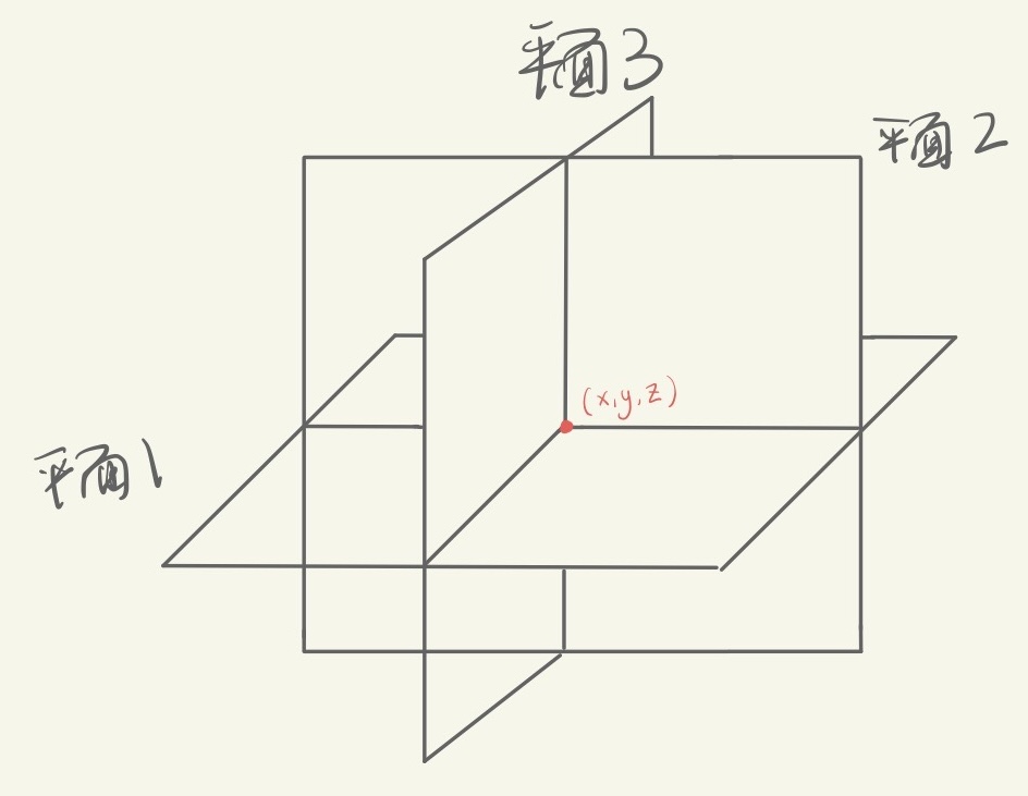
Suppose we have a system of three linear equations in three variables. Each equation can be viewed as the analytic equation of a plane. Solving the system therefore amounts to finding the common intersection of the three planes:

$$A\boldsymbol{x}=\boldsymbol{b} \quad\Longleftrightarrow\quad \begin{cases} a_{11}x+a_{12}y+a_{13}z=b_1,\\ a_{21}x+a_{22}y+a_{23}z=b_2,\\ a_{31}x+a_{32}y+a_{33}z=b_3 \end{cases} \quad\Longleftrightarrow\quad \begin{cases} \boldsymbol{\alpha}_1\cdot\boldsymbol{x}=b_1,\\ \boldsymbol{\alpha}_2\cdot\boldsymbol{x}=b_2,\\ \boldsymbol{\alpha}_3\cdot\boldsymbol{x}=b_3, \end{cases}$$

where $\boldsymbol{\alpha}_1,\boldsymbol{\alpha}_2,\boldsymbol{\alpha}_3$ are the three row vectors of the matrix $A$. Each equation represents a plane in space, and the solution of the system is the common intersection of the three planes. For the coefficient matrix and the augmented matrix, we have

$$r(A\mid\boldsymbol{b})=r(A) \quad\text{or}\quad r(A)+1.$$

The former means that the system has a solution, while the latter means that it has no solution.

If the system is consistent, the dimension of its solution set is

$$\dim\{\boldsymbol{x}:A\boldsymbol{x}=\boldsymbol{b}\}=3-r(A).$$

We can therefore classify the possibilities according to $r(A)=1,2,3$.

$r(A)=1$

Only one of the three row vectors is linearly independent. Without loss of generality, suppose

$$\boldsymbol{\alpha}_2=k\boldsymbol{\alpha}_1, \qquad \boldsymbol{\alpha}_3=m\boldsymbol{\alpha}_1.$$

This means that the normal vectors of the three planes are parallel, so the planes can only coincide or be parallel.

$r(A\mid\boldsymbol{b})=1$: The Three Planes Coincide

In this case, the augmented matrix introduces no additional linearly independent column, and the constants satisfy the same proportional relationships:

$$b_2=kb_1, \qquad b_3=mb_1.$$

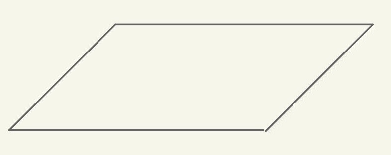
The system can be written as

$$\begin{cases} a_1x+a_2y+a_3z=b_1,\\ ka_1x+ka_2y+ka_3z=kb_1,\\ ma_1x+ma_2y+ma_3z=mb_1. \end{cases}$$

The three equations describe the same plane, so the solution set is that plane. Its dimension is $3-1=2$, and the system has infinitely many solutions.

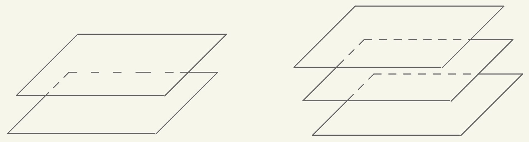
$r(A\mid\boldsymbol{b})=2$: At Least Two Planes Are Parallel but Do Not Coincide

In this case, at least one constant fails to satisfy the original proportional relationship. For example,

$$\begin{cases} a_1x+a_2y+a_3z=b_1,\\ ka_1x+ka_2y+ka_3z=ub_1,\\ ma_1x+ma_2y+ma_3z=wb_1, \end{cases} \qquad u\ne k\quad\text{or}\quad w\ne m.$$

Taking the second plane as an example, divide both sides of its equation by $k$ to obtain

$$a_1x+a_2y+a_3z=\frac{u}{k}b_1.$$

It has the same normal vector as the first plane but a different constant on the right-hand side, so the two planes are parallel and do not coincide. If the direction of $\boldsymbol{\alpha}_1$ is taken as positive, their signed distance is

$$\frac{\left(\frac{u}{k}-1\right)b_1}{\lVert\boldsymbol{\alpha}_1\rVert}.$$

Therefore, the three planes have no common intersection, and the system has no solution.

$r(A)=2$

Exactly two of the three normal vectors are linearly independent. Without loss of generality, suppose $\boldsymbol{\alpha}_1$ and $\boldsymbol{\alpha}_2$ are linearly independent, and let

$$\boldsymbol{\alpha}_3 =p\boldsymbol{\alpha}_1+q\boldsymbol{\alpha}_2.$$

$r(A\mid\boldsymbol{b})=2$: The Three Planes Intersect Along the Same Line

When the system is consistent, the constants must satisfy the same linear relationship:

$$b_3=pb_1+qb_2.$$

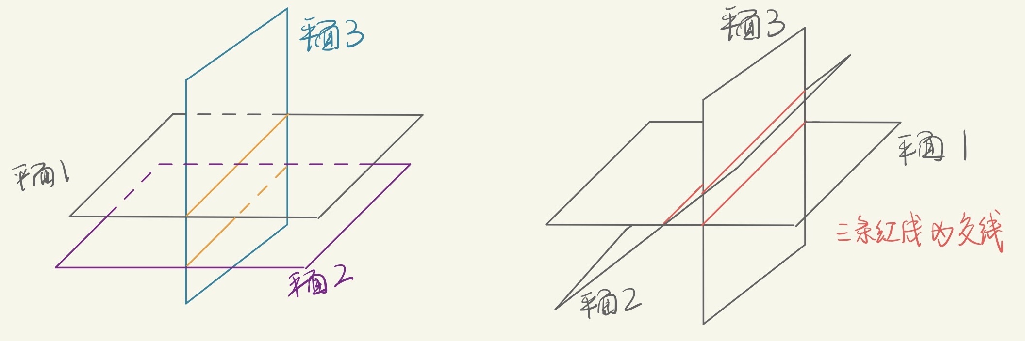
The first two planes intersect along a line, and the third plane contains that line. Therefore, the common intersection of the three planes is a line. The dimension of the solution set is $3-2=1$, so the system still has infinitely many solutions.

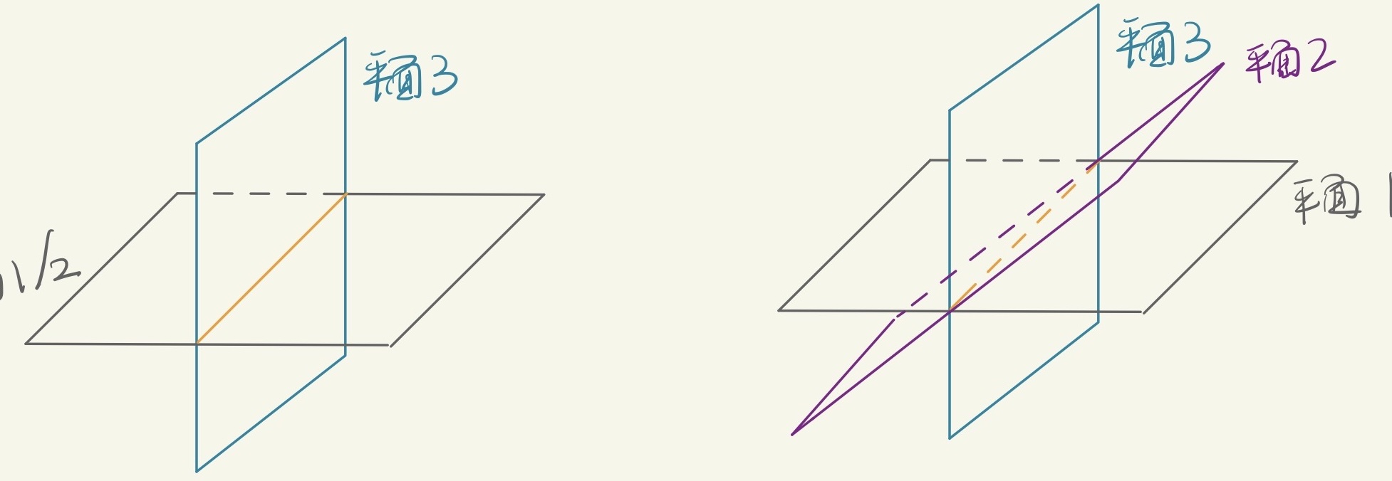
$r(A\mid\boldsymbol{b})=3$: The Three Planes Have No Common Intersection

If

$$b_3\ne pb_1+qb_2,$$

then the third plane has been translated away from the position in which it would contain the intersection line of the first two planes, so it no longer passes through that line. The three planes may intersect pairwise, or two of them may be parallel, but they have no common intersection. Therefore, the system has no solution.

$r(A)=3$

The three normal vectors are linearly independent. Since the augmented matrix has only three rows, we necessarily have

$$r(A\mid\boldsymbol{b})=r(A)=3.$$

The matrix $A$ is invertible, and the system has a unique solution for every $\boldsymbol{b}$:

$$\boldsymbol{x}=A^{-1}\boldsymbol{b}.$$

Geometrically, the three planes intersect at exactly one point, and the dimension of the solution set is $3-3=0$. In particular, when $\boldsymbol{b}=\boldsymbol{0}$, this intersection point is the origin.