Probability Theory

What Is Probability?

When we encounter a discipline—or reconsider one that we learned before but never thought about deeply—we should begin with reality. Think about the many phenomena in the world: which ones cannot be handled by our existing frameworks of knowledge, and why? Is it because those phenomena fall outside the scope of their basic assumptions? Or do those phenomena require more, perhaps even more “outrageous,” assumptions to simplify calculations within our existing frameworks, as long as the required accuracy permits it? (I discussed issues related to disciplines and science in the article Popular Physics: Science and Assumptions.)

The questions above may be too abstract, so let me give a few examples:

• Riding a bicycle to school

In primary and secondary school, we often solve problems like this: the school is 50 km away, and you ride at 50 km/h. How long does it take to arrive?

But the bicycle cannot instantly reach 50 km/h the moment you get on, nor can you still be traveling at 50 km/h when you arrive. So after learning about acceleration, we get an improved version: accelerate first and decelerate later. All right, that is much better.

But you cannot still turn at 50 km/h, can you? There is no such thing as perfectly uniform motion; this model is far too imprecise. So after learning calculus at university, we get another improved version: acceleration depends on how hard the rider pedals, follows a function $f(t)$, and we are asked to find the velocity as a function of time and the time required to arrive. Hmm—much better.

But then the rider falls, bounces and rolls three times on the ground. What is the velocity of their face at the moment it points toward the ground? This is a complicated and admittedly imprecise question, but what I want to show is that, even after learning calculus at university, the previous problems still treated the object as a particle—simply put, they ignored its volume. Yet we often need to study the rotation of the object itself. What then? Students of Theoretical Mechanics receive another lesson from the great scientists: with calculus, Newtonian mechanics, and the assumption of a “rigid body,” we can “simply” describe every motion of a physical object whose deformation can be ignored!

I could keep going, but then I would drift off topic. That discussion should really be about how the many disciplines that appear separate are interconnected and complement one another in explaining the various phenomena of the world. So let us return to the subject: What kinds of problems does probability theory solve? Why can these problems not be solved using calculus, Newtonian mechanics, theoretical mechanics, or even quantum mechanics? What basic assumptions distinguish the objects studied by probability theory from those studied by the disciplines above?

I will explain these questions carefully, but first I want to say this: the questions are more important than the answers. If I have never asked myself these questions, how could I dare say that I understand—or have even studied—this discipline? Even if I received full marks, when someone asks whether I have studied probability theory, all I can say is: I have taken an exam on it.

What is probability? Almost everyone has used dice to make some kind of decision—for example, whoever rolls the lowest number has to go downstairs to pick up the food delivery. That problem is still too complicated, so let us use a coin toss instead. Why do we make decisions this way? Because we believe that no one can determine the result of a coin toss. Although we know it must be either heads or tails, almost all of us also believe that heads and tails should occur about equally often regardless of who tosses the coin. So nobody should care which decision is assigned to heads or tails. But why? Even if a coin cannot be treated as a particle—after all, we must consider rotational motion to obtain heads or tails—it can still be treated as a rigid body. Can we not use the theoretical mechanics discussed above?

The answer is yes! Using theoretical mechanics, as long as we know the coin’s initial position in the hand and the point, magnitude, and direction of the force at the instant it is tossed, we can predict all of its subsequent motion. Of course, we can also know whether it lands heads-up or tails-up. (Careful readers may already have noticed that the hand applies force only when the coin is tossed, while the coin is also affected by gravity, air resistance, and airflow. That brings fluid mechanics into the picture.) Exactly. So if someone uses a vacuum apparatus to toss a coin for you, be cautious: they may very well be able to calculate whether it will land heads or tails. But it is still not that simple. First, several gyroscopes would have to be mounted on the coin to detect its motion, force sensors would have to measure the initial force, and a Bluetooth device would have to transmit the signals to a computer for rapid real-time calculation so that the result could be obtained before the coin lands. Even after all these devices are added, the coin’s center of mass would still have to coincide with its geometric center to preserve symmetry. And this has not yet considered the influence of electromagnetic fields, so an electromagnetic shield could also be added.

After all that, the reader should understand what probability is: the factors affecting an event are so complicated that, in the overwhelming majority of cases, its exact result cannot be predicted before the event ends. At that point, based on symmetry, we may “boldly” predict that all possible outcomes have equal “possibilities” of occurring. That possibility is probability.

P.S. This “equal-probability” assumption based on “symmetry” is extremely widespread. Many physical laws are also based on it, and some may be mentioned below.

What Is a Distribution?

As discussed above, an occurrence may be so complicated that we can only roughly determine what kinds of outcomes are possible, without being able to predict which specific outcome will happen. But if, as stated above, we know nothing and therefore assume that all outcomes have equal probability, does that mean everything we do not understand has the same probability of happening?

I emphasized above that only outcomes that are “symmetric” can be assumed to have equal probability on the basis of symmetry. Take heads and tails again. We do not impulsively assume that heads and tails are equally probable. On the one hand, a coin can approximately be regarded as a centrally symmetric object. On the other hand, it is difficult to determine whether external factors such as wind direction, wind speed, and electromagnetic fields affect heads and tails differently. That is why we assume equal probability.

Now suppose we toss a coin 100 times and want to know the number of heads, or the probability associated with each possible count from 0 to 100. This is still based on tossing a coin. Can we say that the probabilities of 1, 2, …, or 100 heads are all equal? No. Why not? Because we cannot assume such a symmetry. In fact, there is still a certain symmetry: for a fair coin, the probability of obtaining $k$ heads equals that of obtaining $100-k$ heads. For example, 1 and 99 are symmetric, as are 0 and 100. We must therefore begin with the most basic cases that we know are symmetric and reason step by step about the possibility of each outcome above. In many situations, the occurrence we need to consider is composed of these basic symmetric occurrences, but the combination is complex enough to lose some of that symmetry. Different outcomes therefore exhibit different probabilities. When we can infer the probability corresponding to every outcome of this complex occurrence, we say that it follows this “distribution.”

For the same class of occurrences, different points of focus produce different results and therefore different distributions. This gives rise to all kinds of distributions. In fact, they are largely alike, and almost every one of them can even be derived from the act of “tossing a coin.” The normal distribution, which practically everyone has heard of, and the Poisson and exponential distributions, which readers who have not studied probability theory may not have heard of, are all essentially extensions of the coin-toss problem. If we can understand these in the sections that follow, perhaps we will gain a deeper understanding of probability theory.

The Drawing-Lots Model

A bag contains 100 balls: 40 white and 60 black. Twenty balls are drawn in succession. Compare the following four questions:

1. Drawing with replacement, obtain exactly 15 white balls and 5 black balls:

   $$P_1=\binom{20}{15}\left(\frac{40}{100}\right)^{15} \left(\frac{60}{100}\right)^5.$$

2. Drawing without replacement, obtain exactly 15 white balls and 5 black balls:

   $$P_2=\frac{\binom{40}{15}\binom{60}{5}}{\binom{100}{20}}.$$

3. Drawing with replacement, the twentieth ball is white:

   $$P_3=\frac{40}{100}.$$

4. Drawing without replacement, the twentieth ball is white:

   $$P_4=\frac{40}{100}.$$

Question 4 is the “drawing-lots model.” If the results of the preceding draws are unknown, every position in the random ordering is symmetric, and the probability that the ball in position $k$ is white equals the proportion of white balls. We can also imagine randomly placing the 100 balls into 100 positions and examining only position 20. Thus,

$$P_4=\frac{\binom{40}{1}\cdot 99!}{100!}=\frac{40}{100}.$$

Once the preceding results have been observed, the problem becomes one of conditional probability, and the numbers of remaining white balls and remaining balls must be updated accordingly.

What Exactly Is an Event? What Is Conditional Probability?

This section may feel somewhat abrupt. The article has already explained what an event is, so why ask “What is an event?” again? I have found that even when I think I have explained a concept clearly, its abstract nature still allows people to understand it at different depths. Only an in-depth analysis of a relatively “complex” example can often make our understanding of a concept deep and precise. So in this section I will use a “common” exercise to discuss in depth how to describe an event, and then compare and summarize what conditional probability is.

Preface?

Solution 1 is my solution. It uses the same method as Solution 3, although the order of thought and the descriptions of events differ. This difference is precisely the focus of this article. Solution 2 takes a “surprising” approach and was also the inspiration for this article. After understanding this article, you will see that, as long as your reasoning is clear, you can describe an event in any way and solve it using any approach you like. The result will ultimately be correct. You will also find that although correct solutions may appear to use different reasoning, comparing them reveals the same underlying pattern.

Solving the exercise itself is secondary, but understanding its steps and methods is a prerequisite for understanding this article. The solution itself requires the reader to have some foundation in probability theory, but so-called foundations can always be replaced by a clever mind, since these foundations are, after all, the results of clever minds—scientists—thinking about the problems.

Problem

There are two batches containing equal numbers of components. It is known that every product in one batch is qualified, while 25% of the products in the other batch are defective. One product is selected at random from the two batches. It is inspected and found to be qualified, then returned to its original batch. One more product is selected from that same batch. Find the probability that this second product is defective.

Solution 1

---

Let the desired event be $B$. Under the condition that the first product drawn is qualified, let the event that it came from batch $i$ be $A_i$. In the problem, event $B$ describes drawing another product from the original batch. Thus, $B=A_1BUA_2B$. Since $A_1,A_2$ are “mutually exclusive,” we have:

$P(B)=P(A_1B)+P(A_2B)=P(A_1)P(B|A_1)+P(A_2)P(B|A_2)$

The qualification rates of the two batches immediately give:

$P(B|A_1)=0;P(B|A_2)=0.25$

From the discussion above, $A_i$ is an event under a condition. Let the event that the first product is qualified be $X$, and the event that it comes from batch $i$ be $Y_i$.

Clearly, $P(Y_1)=P(Y_2)=0.5$, and $Y_1,Y_2$ are “mutually exclusive” (that is, if $X$ occurs, then either $Y_1$ or $Y_2$ occurs). Therefore, $P(X)=P(XY_1)+P(XY_2)$, and hence:

$A_i=Y_i|X$ $P(A_i)=P(Y_i|X)=\frac{P(XY_i)}{P(X)}$ $P(X)=P(XY_1)+P(XY_2)=P(Y_1)P(X|Y_1)+P(Y_2)P(X|Y_2)$

The qualification rates of the two batches also immediately give:

$P(X|Y_1)=1;P(X|Y_2)=0.75$

Therefore,

$$P(X)=\frac{1}{2}\times1+\frac{1}{2}\times0.75=\frac{7}{8},$$

and hence,

$$P(A_1)=P(Y_1|X)=\frac{4}{7},\qquad P(A_2)=P(Y_2|X)=\frac{3}{7}.$$

Finally, substituting these values into the first equation gives:

$$P(B)=\frac{4}{7}\times0+\frac{3}{7}\times0.25=\frac{3}{28}.$$

Solution 2

---

Let event $A$ be that a product selected at random from the two batches is qualified, and event $B$ be that a second product selected from the original batch is defective. The probability requested by the problem is therefore:

$P(B|A)=\frac{P(AB)}{P(A)}$

Let $W_i$ denote the event that the product comes from batch $i$:

$P(A)=P(AW_1)+P(AW_2)=P(W_1)P(A|W_1)+P(W_2)P(A|W_2)$

Now calculate $P(AB)$:

$AB=W_1AB$ U $W_2AB$. Since $W_1,W_2$ are “mutually exclusive” (the $AB$ here must be distinguished from $B$ and from the desired $B|A$; this will be discussed in detail under Q1 in the Analysis section), we have:

$P(AB)=P(AW_1B)+P(AW_2B)=P(AW_1)P(B|AW_1)+P(AW_2)P(B|AW_2)$

We have $P(AW_i)=P(W_i)P(A|W_i)$, where:

$P(A|W_1)=1;P(B|AW_1)=0;P(A|W_2)=0.75;P(B|AW_2)=0.25$

Substituting these values gives the answer.

Solution 3

---

Let $H_i(i=1,2)$ denote “the first product is drawn from batch $i$,” and let $A$ denote “the product is qualified.” Then:

$P(H_1) =P(H_2)= \frac{1}{2}$

Thus:

$P(A) =P(H_1)P(A|H_1) + P(H_2)P(A|H_2)$

Therefore:

$P(H_1|A)= \frac{P(H)P(A|H_1)}{P(A)}$ $P(H_2|A)==1-P(H_1|A)$

Now let $C_i(i=1,2)$ denote “the second product is drawn from batch $i$.” Then:

$P(\bar{A}) =P(C_1)P(\bar{A}|C_1) +P(C_2)P(\bar{A}|C_2)$

The solution is complete.

Analysis

I will now analyze this problem and its three solutions in a question-and-answer format.

---

Q1: Why does the desired probability become a conditional probability in Solution 2? How does event $B$ in that solution differ from event $B$ in Solution 1 and event $\bar{A}$ in Solution 3?

A1:

First, an event can take different forms when expressed in different ways:

• Event $B$ in Solution 1 is the desired event. Its implicit information is: event $B$ means that, given that the first product drawn is known to be qualified, the second product drawn from the same batch is defective. This is itself an event under the condition of another event.
• There are many similar cases. For example, I can let $W$ be the event of drawing a defective product from the first batch. Then $W$ can also be described as drawing a defective product under the condition that the product is drawn from the first batch. In this sense, $W$ appears to be an event under another event. This problem also contains examples: $X|Y_1$ and $B|A_1$ in Solution 1, and $A|H_1$ and $\bar{A}|C_1$ in Solution 3, correspond to $W/\overline{W}$.
• Looking again at Solution 2, it is not difficult to understand why the desired event is written as $B|A$. One point requires attention, however: the description of event $B$ in Solution 2 may be ambiguous. Does drawing from the original batch already include the condition that $A$ has occurred? After all, the condition given by the problem is precisely that event $A$ occurred. Therefore, the complete description of event $B$ in Solution 2 should be: first select one product at random from the two batches, return it, then select another product from the same batch, with the second product being defective. Notice that the difference from event $B$ in Solution 1 is that event $B$ in Solution 1 includes the occurrence of the event that the first product is qualified.

---

Q2: In Solution 3, event $A$ means drawing a qualified product, but the final expression asks for $\bar{A}$. Should not its probability be $1-P(A)$?

A2:

The explanation here is insufficient and can be regarded as an error. Strictly speaking, event $A$ should mean that a product drawn at random from the two batches is qualified. It is therefore obvious that $\bar{A}$ is not the desired event. The accurate description of the desired event has already been given in the answer to Q1. So this part is indeed wrong.

One point is worth emphasizing: an accurate description of an event is often too complicated, so we tend to abbreviate it. But precisely because of that, a simplified description may mislead our subsequent reasoning and cause the solution to go wrong step by step.

---

What Is Conditional Probability?

Conditional probability is the probability that an event occurs under the condition that another event has occurred. The key is that this condition must itself be a random event. If it is a certain, necessary event, it cannot be called a “condition,” because doing so is meaningless. This statement is difficult to understand, but it is the central point of this article. Let us consider a few examples:

The desired event in the problem has many prerequisites:

• Condition (event) 1: select one product at random from the two batches.

• Condition (event) 2: the selected product is qualified.

• Condition (event) 3: return the selected product.

• Condition (event) 4: select another product from the original batch.

• Condition (event) 5: this final product is defective.

• Implicit condition: the product is returned to and drawn again from the original batch, but we do not know “which” of the two batches that is. (This is easy to understand: only the producer knows which batch is which. As inspectors, we can label them batch 1 and batch 2, but we do not know the qualification rates of the batches bearing those labels.)

When all the conditions above hold, the desired event occurs. Should we define five corresponding events, $A$, $B$, $C$, $D$, and $E$, and write the answer as $E|D|C|B|A$? No. Why?

Because conditions 1, 3, and 4 are definite, necessary events, while only conditions 2 and 5 are random events. Consider condition 1: we select one product from the two batches. We can select only one product—not two and not none—so this is a definite event. Condition 2, however, says that the product selected under condition 1 is qualified. That is not definite, because the product could be defective. Therefore, some “conditions” are restrictions specified by the problem rather than random events. In probability theory, they are not the “conditions” in conditional probability.

For the same reason, “forcing” certain events to serve as conditions can create ambiguity. Consider condition 4 above: selecting another product from the original batch necessarily presupposes conditions 1 and 3. If no product was selected the first time, how could there be an original batch? But matters become easier to explain if we treat a necessary event as part of the random event that follows it:

• Let $A$ = new event 1: select one product at random from the two batches, and the selected product is qualified.
• Let $B$ = new event 2: select one product at random from the two batches, return it, and select another product from the same batch (without knowing which specific batch it is). The final product selected is defective.
• Let $C$ = new event 3: select one product at random from the two batches, and the selected product is qualified. Return it, and select another product from the same batch (without knowing which specific batch it is). The final product selected is defective.

Examine the changes carefully. These “new events” are the most complete descriptions. Of course, there is no need to describe them this carefully when solving an exercise, but it is not worth confusing yourself through abbreviation. Notice that new event 2—the event $B$ above—does not include the condition that the first product is qualified. This $B$ is exactly the $B$ in Solution 2. Event $C=AB$, while the original problem asks for $P(B|A)$. This way of thinking also contains another potential pitfall: “the original batch” means that $A$ intersected with “drawn from the first batch” equals $AB$ intersected with “drawn from the first batch.” In short, whichever approach we take, all roads lead to Rome.

A further question: are events $A$ and $B$ independent? Is $P(AB)=P(A)P(B)$? If we examine event $B$ carefully, we find that it is simply a new occurrence of event $\bar{A}$. In other words, if we do not know whether the first product was qualified, then after returning it, drawing again is effectively the same event as drawing a product directly. Thus, $P(B)=P(\bar{A})$. ?????

Whether this “condition” can be called a random event also depends on the situation. Suppose I have only one batch of products and 25% are defective. Let $K$ be the event that a randomly selected product is defective, so its probability is 0.25. This also occurs under the default condition that I draw from this batch. But because there is only this one batch and I necessarily draw from it, that so-called “condition” is not a random event.

By contrast, in the original problem one product is selected from two batches, so the batch from which it is drawn becomes an uncertain random event. The 25% defect rate of the second batch then becomes a conditional probability: the probability of drawing a defective product under the condition that the product is drawn from the second batch.

Basic Concepts

First, I should explain that I do not like filling an article with technical terms. Unfortunately, many terms in probability theory are highly counterintuitive. If I do not mention them, readers may understand my article perfectly well but become utterly lost when they open a textbook. So I will still explain these basic concepts—that is, the technical terminology.

---

The issue of technical terminology could probably fill an entire article, so I cannot discuss too much of it here. Still, I would like to share a few thoughts: a technical term is a word or symbol that replaces an accurate description of something, for the purpose of simplifying more complex and precise expressions later on.

Technical terms are therefore meaningful. We must express things accurately before we can calculate accurately, and calculate accurately before we can predict or change the laws governing the motion of certain things. Most things in the world can, in essence, be described by basic laws of motion.

For example, if I write $\sin x$, I do not need to explain to someone with relevant professional training what a circle is, what an angle is, how triangles relate to circles, how angles express the relationships between two sides of a triangle, how the trigonometric functions are defined, what basic properties $\sin x$ has, how those properties are proved, and so on.

The problem is that many people who appear to have received the relevant professional training do not understand these technical terms and only know them approximately. Thinking back, I did not understand them when I was at university either. Looking back at university textbooks, I find that they do not explain them; university lecturers do not seem to explain them either. Whether they understand them themselves, I do not know. My purpose in writing this is to encourage future students to think about these basic questions. These concepts and theorems are precisely the most interesting and central questions of a discipline; the point is not merely to memorize them and solve exercises.

Random Events

A random event is one of the possible results of a random experiment.

Here, a “possible result” is a sample point: an indivisible result of the experiment, as mentioned above.

1. A random event is a result.
2. A random event is the result of a particular random experiment.

Random Variables

On the one hand, we want to simplify this form of description further so that we can study its patterns. Whether a coin lands heads or tails, whether a student passes or fails an exam, and whether a light bulb is faulty or functioning all have something in common. How can we describe them abstractly?

On the other hand, some problems are difficult to describe in words. The heights of all people in the world, for example, take almost “continuous” values: there are heights of 166.68556 cm and 166.68557 cm. (We could discuss continuity for a long time. It is another key concept, and the question of how to define it precisely leads to the whole of calculus, which is outside the scope of this article.) How, then, can we write the probability of every possibility or sample point? We can use a function, called the “probability density function.” What does this function mean, and why is it called a density?

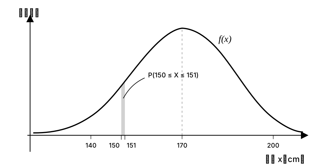
We define the function value to indicate how likely an outcome is near that point. Looking at the figure, for example, it seems obvious that there are more people around 170 cm tall. But this is clearly not a precise statement. An accurate description requires calculus. In the figure, the area of the shaded region is the probability that a person’s height lies between 150 cm and 151 cm. When the interval is very small—for example, from 150 cm to 150.000000001 cm—the probability of falling within it can be approximated as $f(150)\times0.000000001$. This is drifting slightly off topic, but comparison with the density of matter does make the idea understandable: probability per unit of “length” is probability density.

Anyway, the point is that turning verbal descriptions into mathematics allows a large amount of precise information to be expressed concisely, at the cost that everyone must first learn how to read those expressions.

---

A random variable is a special kind of function. Each elementary event—and therefore each event, since events are composed of elementary events—corresponds to a point on the real number line. This rule of correspondence, or function, may be defined arbitrarily by us, as long as it satisfies the required conditions. For example, I can assign heads the value 0 and tails the value 1, or assign heads 1 and tails 2. This is much like code: we abstract a great deal of information into numbers, just as the 26 letters of the English alphabet correspond to numbers in ASCII. The particular implementation of such an assignment has little significance and is mostly conventional.

1. A random variable is a function.
2. The domain of a random variable is the sample space, and its codomain is the real numbers.

Take coin tossing as an example. Define the random experiment as ten independent coin tosses. Then:

1. Obtaining heads five times is a random event.
2. One particular arrangement of heads and tails across the ten tosses is a sample point $w$, or elementary event. The set of all outcomes is the sample space.
3. I assign heads the value 1 and tails the value 2 in each of the ten tosses. For example, the sample point consisting of ten heads can be represented as 1111111111, and so on. Because this representation is one-to-one, it can be written as a function $X(w)$—a random variable. For every $w$, meaning every possible outcome of the ten tosses, this random variable associates one number with it, such as 1111111111 above.
4. The probability mass function of the random variable means that each number $X(w)$ corresponds to an elementary event and therefore to the probability that this elementary event occurs.
5. With the random variable and its distribution above, we can calculate the probability of any event, such as obtaining heads five times—the random event mentioned above. The calculation is simple in principle: find all the elementary events that satisfy the event. For example, heads-heads-heads-heads-heads-tails-tails-tails-tails-tails is one elementary event, because it is a single indivisible outcome. In practice, finding all of them is not so easy.

Population and Sample

What is a population? Definitions in standard textbooks are generally very vague and sometimes even perfunctory. Suppose we want to study human height. We can regard the heights of all human beings as the population—that is, the entirety of the objects under study. What, then, is a sample?

The Relationship Among Population, Sample, Individual, and Random Variable

In intuitive descriptions, it is easy to mix populations, samples, individuals, and random variables together. Strictly distinguishing them places them at two different levels: the objects of study and the probability model.

• An individual is a unit of study and is not itself a random variable.
• Before observation, a characteristic of the $i$th individual can be modeled as a random variable $X_i$.
• A random sample $(X_1,X_2,\ldots,X_n)$ is a random vector. After observation, the resulting $(x_1,x_2,\ldots,x_n)$ is called the observed sample.
• A population may refer to the entire collection of objects under study. Textbooks also commonly use “population $X$” as shorthand for the probability distribution followed by the population characteristic.

Therefore, the question “Is a population or sample a random variable?” cannot be answered simply with “yes” or “no” without context. We should also note that whether a result is unknown depends on the information available to the observer. Suppose I plan to toss a coin 100 times by asking 100 people to toss it once each and then collect the results. From my perspective, before I collect them, the heads-or-tails result of each toss can be described by a random variable. Even if other people have already seen the results, as long as I have not yet obtained those observations, I can still use a probability model to describe my own uncertainty.

Similar experiments may also have entirely different random events and random variables. When studying the joint outcome of 100 coin tosses, each sample point contains the results of all 100 tosses. When studying only one toss, the sample points consist of only heads and tails.

Consider another example: coin tossing. Previously, when we treated the heads-or-tails result as a random variable $X$, that $X$ generally referred to a “particular coin,” which is why we considered an experiment of tossing it $n$ times. But can one coin tell us about all coins? There are two situations:

1. Suppose we want to study coins in a general, universal sense. Each coin is an individual, and its tossing outcome can be represented by a random variable $X_i$. Under the assumptions that the coins are selected randomly and that the tosses are independent and conducted under identical conditions, $X_1,X_2,\ldots,X_n$ form an independent and identically distributed random sample. The specific outcome $x_i$ of each toss is an observation.
2. The other situation is that we study one “special” coin. Each toss is still a random experiment, and its outcome is denoted by the random variable $X_i$. The repeated tosses $(X_1,X_2,\ldots,X_n)$ can be used as a random sample for studying this coin, while the population characteristic is described by the theoretical probability distribution of this coin’s tossing outcomes.

This raises a question: why can coin tossing give rise to these two kinds of population? What about human height?

• Situation 2-1 above corresponds, in the case of human height, to imagining that a person could “start over” and grow to another height. Starting over $n$ times would give a sample. There is also situation 2-2: measure the person’s height repeatedly, with infinitely many measurements constituting the population. But this is not very meaningful, because a person’s height is barely variable over a short period; it is almost a fixed parameter, so repeatedly treating it as a random variable and observing it experimentally has little value. From another perspective, however, this kind of measurement does have some meaning: it tests the randomness of the measurement process. The person’s height is then a constant and also the expectation of the random variable representing the measured height. The object of study has changed, but the problem still falls within probability theory.
• Situation 1 above corresponds to human height as follows: people around the world are the individuals in the population, and the height characteristic of each person can be represented by a random variable $X_i$. When $n$ people are selected at random, $(X_1,X_2,\ldots,X_n)$ is a random sample, and the actually measured height $x_i$ is an observation.

This should make the point clear: when many events involving the same object cannot be made to start over, we can only compare different objects on which the event occurs once. In that case, compared with studying a phenomenon involving one object, the object of study has actually changed, even though the two situations may look similar.

Real measurement and estimation also require us to consider many factors. Therefore, the kind of repeated measurement described in “situation 2-2” is very common in practice. Taking the average of multiple measurements reduces measurement randomness as far as possible, but this should not be confused with the random variable originally under study. (P.S. The sample mean $\bar{X}$ is not equal to the expectation $EX$. The sample mean $\bar{X}$ itself follows a distribution, and only its expectation satisfies $E\bar{X}=EX$. Fully explaining this would take another long discussion.)

Expectation and Variance

If we know the distribution of a random variable, we can “completely” predict it. (Here is a question to leave open: probability is uncertain, yet once we determine its distribution, we determine the probability of every possible result. Is that certain or uncertain? Quantum mechanics introduces this kind of theoretical assumption into physics. In essence, the law is still certain, while the result of a single experiment has a kind of uncertainty—and that uncertainty, the “distribution,” is certain.) I will explain the issues of quantum mechanics in detail in a later popular-physics article.

Sometimes, however, we do not need a complicated probability mass function or distribution function to “understand” a random variable. This is analogous to examinations.

If we knew a student’s accuracy on every exam, exercise, and assignment, the correctness of every solution method they used, and their understanding of every concept in the subject, we could completely determine how well they had mastered that subject. This would clearly be very complicated. Instead, we create an examination paper that covers as many knowledge points and concepts as possible and use it to reflect the student’s mastery of the subject. This inevitably introduces error, but the error is worthwhile in exchange for the time and effort saved. In the same way, we want to give a random variable a kind of “examination paper”—this is expectation and variance.

I do not think the concepts of expectation and variance are particularly difficult to understand. They basically mean what their names suggest. If I discover any problems later, I will add to this section.

Estimation and Testing

Preface

After thinking deeply about estimation and testing, this section will give readers a profound understanding of probability theory!

Since this probability theory article was not written for absolute beginners in the first place, I will now begin directly with formulas. Still, I strongly recommend that students and readers with some foundation continue to the end. If you understand this section, you may gain a great deal from it.

What is estimation? I estimate that most people have never thought carefully about what estimation means. Let me begin with a simple example. (This is not an analogy; it really is an example.)

“I estimate that Trump is not a good person.” There is nothing wrong with this sentence. But if you say, “Trump is not a good person,” that is a much bigger problem. This is a complex random event. If you claim it is a necessary event, I must remind you that there are almost no necessary events in the real world. Even “every human being in the world is either male or female” is not a necessary event. This is drifting off topic. In short, a necessary event is an idealized case.

So how do I estimate that Trump is not a good person? Is the estimate credible? First, I would have to state the probability that Trump is not a good person. How could I obtain that probability? I would need a distribution and a sample. A distribution would require an accurate definition of a good person—and it should be a quantitative definition rather than a simple good-or-bad division. We would need to identify human characteristics and the probability that someone with those characteristics is a good person, such as the probability that their “good-person score” exceeds some value $b$.

This is an extremely complicated process, but we can imagine how it might work. For example, I once heard someone say, “People with big noses are cut out to be officials.” We cannot make a claim like that casually. To speak in terms of probability, this event is much simpler than whether Trump is a good person. We could measure the dimensions of the noses of as many people in the world as possible and use their average as a reference point. Then we could calculate the average nose dimensions of officials and compare them with that reference. But that gives us only the mean. We would also need the variance of officials’ nose dimensions, and would even have to quantify official rank—how senior an official is—and then calculate the relationship between officials’ noses and the level of their positions, and so forth.

Although I have not conducted these experiments, my wild guess is that the relationship is about as likely as my being elected president of the United States. (Notice that “wild guess” is the precise phrase. I cannot call this an estimate, because I have neither a theory nor an experiment. I am simply guessing.) All right, now for the main discussion.

Main Discussion

Estimation means deriving the distributions that the sample mean and sample variance should follow from an assumed original distribution, and then using the sample mean to infer the probability that the expectation—or another parameter—of the original distribution lies within a certain range.

The assumed original distribution is the “distribution of good people” in the preface. Clearly, it would be the distribution of a function of a complex multidimensional random variable. The sample consists of Trump’s behavior that we have observed, while the population is obviously all of Trump’s behavior and thoughts, which is also a relatively accurate way to define a person. Inferring the probability that Trump is a good person from the behavior observed so far is estimation.

• Question: If we already know the original distribution, why must we infer its expectation?
• Answer: More precisely, we know the type of the original distribution but not its exact parameters. For example, suppose we know that the “population” to be tested—the random variable $X$ corresponding to the population—follows an exponential distribution, but we do not know $\lambda$. We then use the expression for the exponential distribution to determine the distributions followed by the sample mean and variance. Note that those distributions depend on the original parameter $\lambda$ and often on the original expectation $EX$. We then use those distributions and the measured values to work backward and infer the $\lambda$ of the original exponential distribution.

The exponential-distribution example above would be complicated. Certain properties of the normal distribution, however, make the calculation simpler. The normal distribution also has a degree of universality because of the central limit theorem. Therefore, university courses only require students to master cases in which the original distribution is normal. I will likewise use the normal distribution as my example:

According to the central limit theorem, should not the sample mean Xbar of an exponential distribution and the sample mean Xbar of a normal distribution both follow a normal distribution?

The central limit theorem requires $n\to\infty$, meaning that the sample space must be infinite. In actual testing, however, the samples we draw are always “small” in number. The normal distribution has a special property: for any $n$, the sample mean still follows a normal distribution.

---

This section gives the detailed derivation of interval estimation for a normal distribution. Some details may be omitted because they are all available in textbooks. In addition, since some platforms do not support LaTeX, I will sometimes use Xbar to represent the sample mean of $X$.

Let $X_1,X_2,\ldots,X_n$ be independent and identically distributed, with $X_i\sim N(\mu,\sigma^2)$. Then the sample mean satisfies

$$\overline{X}=\frac{1}{n}\sum_{i=1}^{n}X_i \sim N\left(\mu,\frac{\sigma^2}{n}\right).$$

A random variable such as $X$ could represent the brightness of light bulbs produced by a factory, and it is quite reasonable for it to follow a normal distribution. We now take $n$ light bulbs. The brightness of the $i$th bulb is $X_i$, and the average brightness of the $n$ bulbs is also a random variable, Xbar. Notice that this refers to brightness before measurement; as with a coin toss, we do not know how bright it is. From the assumption that the brightnesses of these $n$ bulbs are independent and identically distributed, together with a series of other “fancy maneuvers,” we obtain the distribution function of Xbar shown above. (The proof is in the textbooks.) Its graph is shown below:

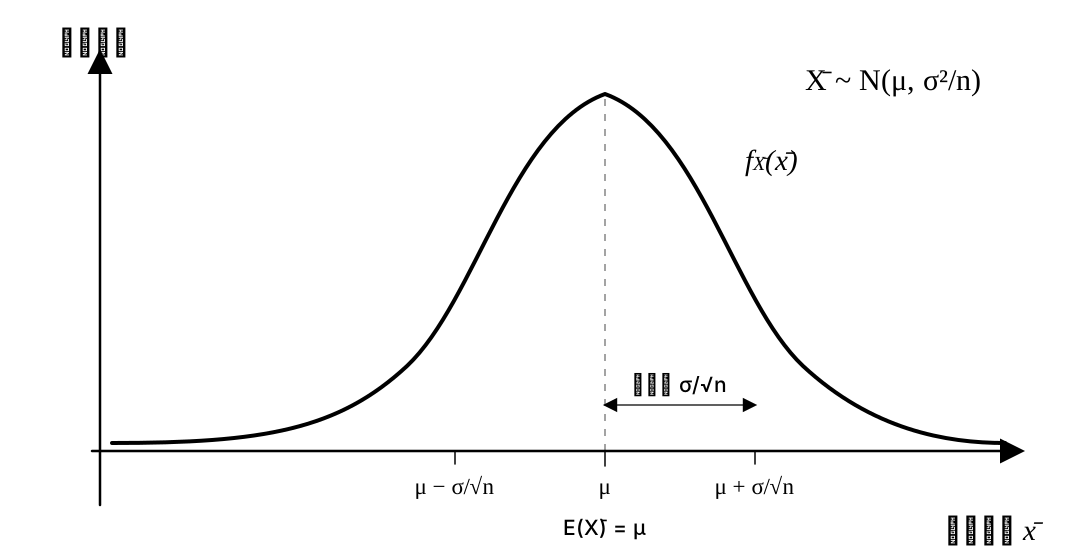
In the usual textbook situation—like coin tossing—we know $\mu$ and are asked for the probability that a measured value of Xbar lies in some range. We often solve problems like this. But this is not the usual real-world situation at all! How could we know the expected brightness of the light bulbs produced by the factory? We cannot. We inspect them precisely because we do not know it. Why inspect anything if we already know everything?

So in the truly usual situation, we do not know $\mu$. We select several bulbs, measure them, and take their mean. Does that mean the result is $\mu$? Certainly not. This helps us understand the meaning of the distribution of Xbar: the mean brightness of the $n$ selected bulbs has expectation $\mu$ and variance $\sigma^2/n$. It also fluctuates, and values near $\mu$ have higher probability, as shown in the figure.

But how can we use Xbar to estimate $\mu$? They are not equal. We already have the distributions they follow, meaning that we know their probability in any interval. If we “simplify” Xbar, the situation becomes clearer:

$$Y=\frac{\overline{X}-\mu}{\sigma/\sqrt{n}}\sim N(0,1).$$

Given a significance level $\alpha$, choose the critical value $\Delta_\alpha$ such that

$$P\left\{|Y|<\Delta_\alpha\right\}=1-\alpha.$$

Substituting the definition of $Y$ gives

$$P\left\{ \overline{X}-\Delta_\alpha\frac{\sigma}{\sqrt{n}} <\mu< \overline{X}+\Delta_\alpha\frac{\sigma}{\sqrt{n}} \right\}=1-\alpha.$$

Therefore, after measuring the sample mean $\overline{x}$, an interval estimate for $\mu$ with confidence level $1-\alpha$ is

$$\left( \overline{x}-\Delta_\alpha\frac{\sigma}{\sqrt{n}}, \overline{x}+\Delta_\alpha\frac{\sigma}{\sqrt{n}} \right).$$

That completes the interval estimation.

---

But this may look confusing:

1. Xbar is clearly a variable, so why has $\mu$ become a variable?
2. The measured Xbar cannot represent all possible Xbar values. How can one value of $X$ be used to determine the probability of $\mu$?
3. We do not even know $\mu$, yet somehow we know—and know exactly—$\sigma$? Is that not nonsense?

• On question 1: Why do we know $\mu$? In fact, we never do! Throughout history, humans have taken experimental results $X$ that approach some value and then devised a theory $A$ to explain where the theoretical value $\mu$ comes from. Theory $A$ is the distribution function. Moreover, $\mu$ and Xbar are variables on an equal footing. If we can accept $\mu$ as a constant, why “look down on” Xbar? We will return to this in the answer to question 2. At this point, we can think about the coin-toss problem again—and again and again. We will discover that we do not know $EX=\mu=0.5$. It is merely the experimental Xbar values accumulated over many years that show it to be very close to 0.5. We therefore believe, or assume, that in the ideal case $\mu$ is 0.5. Yet many textbooks reverse cause and effect: they present an inferred result as fact, make the experimental results appear “frivolous,” and do not mention this process of thought and inference at all!
• On question 2: This is indeed not rigorous. Therefore, we often measure several groups and roughly regard the measurement results as accurate. More precisely, if we assume that the distribution is fixed—even though distributions themselves always contain deviations—we can determine only the relationship between the sample mean Xbar and the expectation $\mu$ of the assumed original distribution.
• On question 3: Indeed. In practice, another “more reliable” testing method is used: a test based on the $t$ distribution. The population standard deviation $\sigma$ is replaced by the sample standard deviation $S$, and after simplification the resulting statistic follows a $t$ distribution. This leaves only the population expectation $\mu$ unknown and therefore makes the test more accurate.

A Brief Discussion of Point Estimation

Point estimation can be understood as a simplified—and less accurate—form of interval estimation.

Point estimation is often used to estimate other parameters, such as $\lambda$. In the overwhelming majority of cases, however, such a parameter is a function of the expectation $\mu$. We could actually use interval estimation to estimate a range in which $\mu$ takes values with “high probability,” then use properties such as monotonicity to solve for an interval of the desired parameter $\lambda$. This would be more accurate, but perhaps also more complicated. In any case, it is not required by the syllabus, though this point still needs to be understood.

Several Common Distributions and Their Meaning

The discussion above shows that different experiments correspond to different distributions. In nature and society, many experiments follow surprisingly similar distributions. What are some typical distributions, and what kinds of experiments make them display similar or different distributional patterns?

Binomial Distribution

Many experiments begin with this simple one: toss a coin independently and repeatedly $N$ times and ask for the probability of obtaining heads $k$ times. As mentioned above, the same pattern applies if a batch contains $N$ light bulbs with a 1% failure rate and we ask for the probability that $k$ bulbs are qualified.

This article will not state or calculate the specific distribution functions, because any textbook explains them clearly. Instead, I want to supplement them with certain issues that textbooks and even teachers overlook.

Poisson Distribution

We often hear statements such as: a certain place receives an average of 100,000 visitors per day during a holiday. We can assume that every extremely small time interval during this period—say 1 ms—is an independent “coin toss”: either one person passes by or no one does. The probability is then $100000/(24\times60\times60\times1000)=0.116\%$. This is therefore a binomial distribution with $N=24\times60\times60\times1000$ trials. We can use it to predict the probability that 80,000 people will visit tomorrow.

When $N$ is very large and $Np$ is not large, a few techniques from calculus can be used to approximate this distribution function, producing the Poisson-distribution formula found in textbooks today.

Applications of the Poisson Distribution

Just as the environment may differ from one coin toss to another—for example, a magnet might be placed next to the coin during ten of the tosses—random phenomena that can be explained using a Poisson distribution must satisfy its basic assumptions: every extremely small interval of “time” or “space” is independent of the others and symmetrically follows the same “coin-toss” distribution.

At the beginning of this article, we emphasized the importance of the real environment. Sometimes a coin toss can be treated as a mechanics problem with an exact solution. In most situations, however, there are too many influencing factors for us to calculate—or for us actually to have calculated—the result, so we treat it as a random experiment. Similarly, treating the outcomes of different coin tosses as independent random events assumes that the factors influencing them have hardly changed.

What if they have changed? On a summer holiday, for example, evenings may be cooler and therefore attract more visitors. This fails to satisfy the Poisson assumptions above, and using the Poisson distribution to predict the probabilities of a series of related events would then be wrong.

(We might even abandon the coin-toss-style distinction between right and wrong and instead discuss the degree of accuracy. This idea is extremely widespread and important in every field of science and technology: discussing right and wrong without considering accuracy and cost is meaningless. Concepts in calculus such as continuity, “infinitesimals,” and differentiability cannot exist in reality. Compared with a 1 cm difference in height, however, a 1 nm difference can be treated as “infinitesimal,” and so on.)

Exponential Distribution

The exponential distribution is related to the Poisson distribution above, but our focus is different. We consider the same random experiment but a different random event. This time, we want to know: if no person arrives for a continuous period of length $t$ and then someone finally arrives, what is the probability? This question is easy. The number of trials changes, all preceding outcomes are non-occurrences, and we calculate the probability. It can be derived from a classical probability problem with a little calculus.

The Memorylessness of the Exponential Distribution?

The exponential distribution does have this property. Consider the lifetime of a light bulb. Suppose we observe one bulb and assume that its failure rate is fixed—say 1%. We can use the model above to describe it. We then obtain the following conclusion: if the bulb has already been used for ten years without failing, its probability of failing next is the same as when it was brand-new. This is the so-called memoryless property. It strongly violates common sense, yet some teachers and textbooks use precisely this example. It is clearly wrong. So I will explain what is wrong with it and where the real-world significance of this property lies.

The problem is the initial assumption: every extremely small time interval during the period is assumed to be an independent event. Thus, whether the bulb fails in this interval has no relationship with whether it fails in the next interval—or even ten thousand intervals later. But is that actually true? Of course not. The bulb’s components are consumable. As the bulb is used, wear accumulates and increases the probability of failure, so its failure rate is not constant.

Clearly, this does not mean that science has proved a phenomenon contrary to common sense. It means that the scientific assumption does not apply in this case. Are there cases in which it does apply? Yes: atomic decay. A detailed explanation would take us off topic again, but I will briefly describe the issue.

Many kinds of matter—including human beings—experience “wear” over time. At root, this is a process of increasing entropy in thermodynamics. Entropy itself is defined only for large numbers of particles, because thermodynamic problems can, somewhat imprecisely, be understood as problems involving probability distributions over large numbers of particles. Atoms, especially larger atoms—I will not explain here why “larger” atoms are less stable and more likely to “decay,” or in other words to be radioactive—have a certain probability of decaying. Decay can be understood simply as an atom splitting internally and releasing smaller particles and energy, meaning light. There is no evidence that this probability depends on how long the atom has “survived.” This can also be understood from the perspective of entropy: an atom contains very few elementary particles and does not belong to the thermodynamic domain, just as a single electron does not have a temperature. (It is fine if this is difficult to follow; it contains a great deal of information.) Anyway, atomic decay has at least a much weaker relationship with elapsed time than light-bulb failure does, so it is more suitable for description by an exponential distribution.

P.S. Why is atomic decay treated as a random event? This is physics! Think back to the essence of probability discussed at the beginning. Exactly: it is entirely possible that humanity simply has not yet discovered its law and can therefore only treat it as a random event. Physics can certainly explain a great deal—as can other scientific fields—but there is even more that it cannot explain. As the saying goes, the more we know, the more we realize we do not know. But, but, but: every science has one thing in common. If an experiment refutes my theory, then the theory must be the problem. That is what it means to respect facts.

Normal Distribution

Wow, here is another remarkable distribution—perhaps the “most remarkable” of all. Readers may have heard that the grades of students in a class follow a normal distribution: few students receive very high or very low scores, while many receive scores in the middle. Some schools even require final grades to conform to this distribution, forcing teachers to “adjust” students’ grades artificially so that they follow it. That is simply ridiculous.

Anyway, the normal distribution begins with the central limit theorem. It addresses the following issue: the average of individuals from any population will cluster around the expectation of the population—that is, of the random variable corresponding to the population—and its specific distribution is the Gaussian distribution function.

The statement above is admittedly not human-friendly. In other words, if we have many random variables that are mutually independent and follow the same distribution, their average follows a normal distribution.

For example, toss a coin many times. The heads-or-tails result, represented as 1 or 0, of each toss is independent and follows the same distribution—let us call it the 0/1 distribution. Therefore, the average of the 1/0 results across all those tosses follows a normal distribution, whose expectation is precisely the expectation of the 0/1 distribution: 0.5. Thus, not every arbitrary random variable follows a normal distribution. We first need multiple independent and identically distributed random variables, and what we care about is their average. The universality of the normal distribution is the main focus of the next section.

The Universality of the Normal Distribution?

To understand why the normal distribution has this form, we must return to entropy. A proper discussion of entropy would take us off topic again, so I will leave a question open: among distributions with a known mean and variance, the normal distribution has the maximum entropy. Interested readers can prove this themselves.

The general applicability of the normal distribution is also often exaggerated. Independence and identical distribution are in fact extremely demanding requirements. Random variables often have strong correlations, and such correlations inevitably make the normal distribution vanish like a mirage. Consider the examination-grade example above. The distribution of grades in a class depends to a large extent on the teacher’s teaching ability, attitude, and style. A conscientious teacher may deliberately remind students who are not paying attention and may use a humorous style that arouses their interest. The resulting distribution will inevitably differ from that produced by a master of reading directly from PowerPoint slides. The grades of students around the entire world may be more likely to follow a normal distribution, but requiring the grades of one class to do so is absurd and reverses cause and effect.

The conclusion can always be turned around yet again. In university probability courses, the chapter on mathematical statistics is built on the normal distribution. What justification is there for that?

When a sample does not follow a normal distribution, the mean of a “large” sample will always follow a normal distribution because of the central limit theorem. But here is the question: the sample mean follows a normal distribution, yet it is not the original random variable connected to the population. What problem does this cause?